진행상황 tqdm

패키지 설치를 할 때 보면 나오는 텍스트 타입의 진행바 모양이 있다. 작업이 어느 정도 진행되었고 남았는지 알 수 있어서 없는 것보다는 답답함이 해결되는 효과가 있다.

이것을 구현하기 위해서는 tqdm 패키지를 사용하면 된다. tqdm의 파라미터로 iterable 객체를 넣어주면 알아서 전체 반복 횟수 중 진행반복횟수를 표시해 준다.

from tqdm import tqdm
import time
for i in tqdm(range(100)):
   time.sleep(0.01)

콘솔 출력문을 추가했을 경우 아래와 같이 된다. (없으면 한 줄로 업데이트 진행됨)

• range(30, 100) 으로 파라미터를 줄 경우, 전체 반복량은 70이므로 0/70부터 시작하여 70/70까지 진행 표시된다.

파라미터 설명

• iterable : 반복자 객체
• desc : 진행바 앞에 텍스트 출력
• total : int, 전체 반복량
• leave : bool, default로 True. (진행상태 잔상이 남음)
• ncols : 진행바 컬럼길이. width 값으로 pixel 단위로 보임.
• mininterval, maxinterval : 업데이트 주기. 기본은 mininterval=0.1 sec, maxinterval=10 sec
• miniters : Minimum progress display update interval, in iterations.
• ascii : True로 하면 '#'문자로 진행바가 표시됨.
• initial : 진행 시작값. 기본은 0
• bar_format : str

• 전체 작업량을 알고 있고, 처리된 량으로 진행바를 표시할 경우. (update에 진행량을 파라미터로 추가). 파일 읽기 같은 경우 활용가능하다.

t = tqdm(total=500)
for i in range(250):
    time.sleep(0.01)
    t.update( 2 )
t.close()

• clear() : 삭제

• refresh() : 강제 갱신

• 중간부터 진행되는 경우. 전체 작업량이 500인데, 100은 이밎 처리되서 100부터 시작하는 경우.

t = tqdm(total=500, initial=100, ascii=True)
for i in range(200):
    time.sleep(0.01)
    t.update( 400/200 )
t.close()

Written with StackEdit.

Upload File to Google Drive

Prepare

구글 사이트에서 준비 작업이 필요하다.
https://console.developers.google.com/flows/enableapi?apiid=drive
프로젝트 생성
Google Drive API 사용.
Credential에서 OAuth 화면.
Product Name 입력.
json 파일 다운 로드 (client_drive.json).
작업디렉터리로 파일 이동.

# 파이썬 패키지 설치
pip install google-api-python-client

토큰 생성

from googleapiclient.discovery import build
from httplib2 import Http
from oauth2client import file, client, tools

scopes = 'https://www.googleapis.com/auth/drive.file'
store = file.Storage('storage.json')
creds = store.get()

try :
    import argparse
    flags = argparse.ArgumentParser(parents=[tools.argparser]).parse_args()
except ImportError:
    flags = None

if not creds or creds.invalid:
    print('make new cred')
    flow = client.flow_from_clientsecrets('client_drive.json', scopes)
    creds = tools.run_flow(flow, store, flags) if flags else tools.run_flow(flow, store)

콘솔로 위의 파일을 실행하면, 웹브라우저가 뜨고, 구글 인증/로그인을 하면 된다. 현재 폴더에 storage.json 이라는 토큰이 생김. 보안 파일이므로 중요보관.

파일 업로드

from oauth2client.client import GoogleCredentials
from googleapiclient.discovery import build
from httplib2 import Http
from oauth2client import file, client, tools

store = file.Storage('storage.json')
creds = store.get()
drive = build('drive', 'v3', http=creds.authorize(Http()))
uploadfiles=( ('a.txt'),)
for f in uploadfiles:
    fname = f
    metadata={'name':fname, 'mimeType':None}
    res = drive.files().create(body=metadata, media_body=fname).execute()
    if res:
        print('upload %s'%fname)
        

파일 다운로드

파일ID는 구글드라이브에서 해당 파일 공유하기해서 링크 주소를 얻어오면 id값이 들어있다.

import io
from apiclient.http import MediaIoBaseDownload

results = drive.files().list(pageSize=10,fields="nextPageToken, files(id, name)").execute()
items = results.get('files', [])
if not items:
    print('No files found.')
else:
    print('Files:')
    for item in items:
        print(item)
        print('{0} ({1})'.format(item['name'], item['id']))

#https://drive.google.com/open?id=1SY8FS1QcGTknYJjEUgaqj1ucWEtESTn3
# request = drive.files().export_media(fileId='a.txt', mimeType=EXCEL)
request = drive.files().get_media(fileId='1SY8FS1QcGTknYJjEUgaqj1ucWEtESTn3')
fh = io.FileIO('b.txt', 'wb')
downloader = MediaIoBaseDownload(fh, request)
done = False
while done is False:
    status, done = downloader.next_chunk()
    print('Download %d%%.' % int(status.progress() * 100))
        

CoLab에서 구글 드라이브 파일 가져오기

# Install the PyDrive wrapper & import libraries.  
# This only needs to be done once per notebook. 
!pip install -U -q PyDrive 
from pydrive.auth import GoogleAuth 
from pydrive.drive import GoogleDrive 
from google.colab import auth 
from oauth2client.client import GoogleCredentials 

# Authenticate and create the PyDrive client.  
# This only needs to be done once per notebook. 
auth.authenticate_user() 
gauth = GoogleAuth() 
gauth.credentials = GoogleCredentials.get_application_default() 
drive = GoogleDrive(gauth) 

# Download a file based on its file ID.  
#  
# A file ID looks like: laggVyWshwcyP6kEI-y_W3P8D26sz 
file_id = 'REPLACE_WITH_YOUR_FILE_ID' 
downloaded = drive.CreateFile({'id': file_id}) print('Downloaded content "{}"'.format(downloaded.GetContentString()))  

  

Written with StackEdit.

Fourier Transform

푸리에 변환

푸리에 변환은 연속적인 시계열 데이터를 sin, cos 함수들과 같은 파형들의 합으로 나타내는 것으로 여러 개의 주파수 성분들로 분해하는 작업이다.
주로 신호 처리나 사운드, 이미지와 같은 데이터의 주파수 변환에 많이 사용한다.
그렇다면 어떻게 분해를 할 수 있는 것일까?
여기서는 이론적인 이해가 아닌 프로그래밍 구현측면에서 접근하도록 한다.

위 그림은 도형 이미지를 시간에 따른 x, y 좌표 리스트로 나누어 x, y 각각을 주파수 분해한 다음 분해된 주파수들을 하나씩 결합하여 그린 모양이다. 주파수를 하나씩 더 했을 때 점점 원본에 닮아가는 것을 확인할 수 있다.
노이즈가 섞인 원본 신호라면 주파수 분해 후 적절한 신호의 재결합을 통해 노이즈가 제거되는 효과도 나타날 수 있을 것이다.

도구

가장 쉽게 접근할 수 있는 것은 python의 numpy나 scipy 라이브러리로 쉽게 원하는 작업을 할 수 있다. cpp로 된 라이브러리도 google에서 검색하면 금방 찾을 수 있다.

해결하려는 문제

시계열 데이터를 주파수 성분으로 분해하고 분해된 수치 정보만으로 원본을 복구하는 작업을 수행하고자 한다.

알 수 없는 시그널

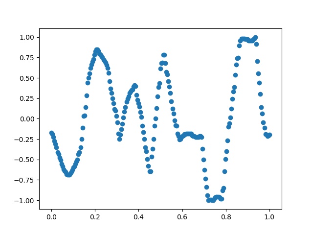
시간값과 신호크기만 있는 시계열 데이터가 있다고 하자.

'''  
foutier transform  
'''  
  
import numpy as np  
import matplotlib.pyplot as plt  
  
txlist = [(0.0, -0.1729957805907173), (0.0045871559633027525, -0.189873417721519), (0.009174311926605505, -0.2236286919831224), (0.013761467889908258, -0.2742616033755274), (0.01834862385321101, -0.3080168776371308), (0.022935779816513763, -0.3502109704641351), (0.027522935779816515, -0.4092827004219409), (0.03211009174311927, -0.4345991561181435), (0.03669724770642202, -0.47679324894514763), (0.04128440366972477, -0.510548523206751), (0.045871559633027525, -0.5527426160337553), (0.05045871559633028, -0.5864978902953586), (0.05504587155963303, -0.620253164556962), (0.05963302752293578, -0.6371308016877637), (0.06422018348623854, -0.6540084388185654), (0.06880733944954129, -0.6793248945147679), (0.07339449541284404, -0.6877637130801688), (0.0779816513761468, -0.6877637130801688), (0.08256880733944955, -0.6877637130801688), (0.0871559633027523, -0.6708860759493671), (0.09174311926605505, -0.6540084388185654), (0.0963302752293578, -0.6286919831223629), (0.10091743119266056, -0.5949367088607596), (0.10550458715596331, -0.5864978902953586), (0.11009174311926606, -0.5527426160337553), (0.11467889908256881, -0.5274261603375527), (0.11926605504587157, -0.5021097046413502), (0.12385321100917432, -0.4345991561181435), (0.12844036697247707, -0.4092827004219409), (0.13302752293577982, -0.3502109704641351), (0.13761467889908258, -0.24894514767932485), (0.14220183486238533, -0.11392405063291144), (0.14678899082568808, 0.029535864978903037), (0.15137614678899083, 0.03797468354430378), (0.1559633027522936, 0.139240506329114), (0.16055045871559634, 0.28270042194092837), (0.1651376146788991, 0.4430379746835442), (0.16972477064220184, 0.5021097046413503), (0.1743119266055046, 0.5527426160337552), (0.17889908256880735, 0.620253164556962), (0.1834862385321101, 0.6624472573839661), (0.18807339449541285, 0.6962025316455696), (0.1926605504587156, 0.729957805907173), (0.19724770642201836, 0.7805907172995781), (0.2018348623853211, 0.8227848101265822), (0.20642201834862386, 0.8481012658227849), (0.21100917431192662, 0.8481012658227849), (0.21559633027522937, 0.8312236286919832), (0.22018348623853212, 0.7974683544303798), (0.22477064220183487, 0.7890295358649788), (0.22935779816513763, 0.7721518987341771), (0.23394495412844038, 0.7552742616033756), (0.23853211009174313, 0.7215189873417722), (0.24311926605504589, 0.7046413502109705), (0.24770642201834864, 0.6877637130801688), (0.25229357798165136, 0.6540084388185654), (0.25688073394495414, 0.620253164556962), (0.26146788990825687, 0.5611814345991561), (0.26605504587155965, 0.4599156118143459), (0.2706422018348624, 0.36708860759493667), (0.27522935779816515, 0.31645569620253156), (0.2798165137614679, 0.24894514767932496), (0.28440366972477066, 0.1898734177215189), (0.2889908256880734, 0.11392405063291133), (0.29357798165137616, 0.09704641350210963), (0.2981651376146789, 0.029535864978903037), (0.30275229357798167, -0.04641350210970463), (0.3073394495412844, -0.18143459915611815), (0.3119266055045872, -0.24894514767932485), (0.3165137614678899, -0.19831223628691985), (0.3211009174311927, -0.13080168776371304), (0.3256880733944954, -0.06329113924050633), (0.3302752293577982, 0.012658227848101333), (0.3348623853211009, 0.08860759493670889), (0.3394495412844037, 0.139240506329114), (0.3440366972477064, 0.2067510548523206), (0.3486238532110092, 0.240506329113924), (0.3532110091743119, 0.2742616033755274), (0.3577981651376147, 0.31645569620253156), (0.3623853211009174, 0.33333333333333326), (0.3669724770642202, 0.35021097046413496), (0.37155963302752293, 0.3586497890295359), (0.3761467889908257, 0.39240506329113933), (0.38073394495412843, 0.40928270042194104), (0.3853211009174312, 0.4008438818565401), (0.38990825688073394, 0.2911392405063291), (0.3944954128440367, 0.23206751054852326), (0.39908256880733944, 0.1898734177215189), (0.4036697247706422, 0.14767932489451474), (0.40825688073394495, 0.08016877637130793), (0.41284403669724773, 0.021097046413502074), (0.41743119266055045, -0.08860759493670889), (0.42201834862385323, -0.16455696202531644), (0.42660550458715596, -0.24894514767932485), (0.43119266055045874, -0.3502109704641351), (0.43577981651376146, -0.4008438818565401), (0.44036697247706424, -0.49367088607594933), (0.44495412844036697, -0.5780590717299579), (0.44954128440366975, -0.6455696202531646), (0.4541284403669725, -0.6455696202531646), (0.45871559633027525, -0.4683544303797469), (0.463302752293578, -0.36708860759493667), (0.46788990825688076, -0.24894514767932485), (0.4724770642201835, -0.08860759493670889), (0.47706422018348627, 0.00421940928270037), (0.481651376146789, 0.13080168776371304), (0.48623853211009177, 0.2742616033755274), (0.4908256880733945, 0.38396624472573837), (0.4954128440366973, 0.4345991561181435), (0.5, 0.6118143459915613), (0.5045871559633027, 0.6793248945147679), (0.5091743119266054, 0.6877637130801688), (0.5137614678899083, 0.7805907172995781), (0.518348623853211, 0.7805907172995781), (0.5229357798165137, 0.6793248945147679), (0.5275229357798165, 0.5696202531645569), (0.5321100917431193, 0.5443037974683544), (0.536697247706422, 0.4599156118143459), (0.5412844036697247, 0.39240506329113933), (0.5458715596330275, 0.31645569620253156), (0.5504587155963303, 0.21518987341772156), (0.555045871559633, 0.1223628691983123), (0.5596330275229358, 0.06329113924050622), (0.5642201834862385, -0.021097046413502074), (0.5688073394495413, -0.08016877637130804), (0.573394495412844, -0.08860759493670889), (0.5779816513761468, -0.18143459915611815), (0.5825688073394495, -0.21518987341772156), (0.5871559633027523, -0.2573839662447257), (0.591743119266055, -0.24894514767932485), (0.5963302752293578, -0.2236286919831224), (0.6009174311926605, -0.21518987341772156), (0.6055045871559633, -0.2067510548523207), (0.6100917431192661, -0.189873417721519), (0.6146788990825688, -0.189873417721519), (0.6192660550458715, -0.18143459915611815), (0.6238532110091743, -0.18143459915611815), (0.6284403669724771, -0.18143459915611815), (0.6330275229357798, -0.18143459915611815), (0.6376146788990825, -0.18143459915611815), (0.6422018348623854, -0.18143459915611815), (0.6467889908256881, -0.2067510548523207), (0.6513761467889908, -0.21518987341772156), (0.6559633027522935, -0.21518987341772156), (0.6605504587155964, -0.2236286919831224), (0.6651376146788991, -0.2236286919831224), (0.6697247706422018, -0.2236286919831224), (0.6743119266055045, -0.2236286919831224), (0.6788990825688074, -0.21518987341772156), (0.6834862385321101, -0.21518987341772156), (0.6880733944954128, -0.2236286919831224), (0.6926605504587156, -0.36708860759493667), (0.6972477064220184, -0.5021097046413502), (0.7018348623853211, -0.6286919831223629), (0.7064220183486238, -0.7383966244725738), (0.7110091743119266, -0.8396624472573839), (0.7155963302752294, -0.9409282700421941), (0.7201834862385321, -1.0), (0.7247706422018348, -0.9915611814345991), (0.7293577981651376, -0.9915611814345991), (0.7339449541284404, -0.9915611814345991), (0.7385321100917431, -1.0), (0.7431192660550459, -1.0), (0.7477064220183486, -0.9831223628691983), (0.7522935779816514, -0.9662447257383966), (0.7568807339449541, -0.9578059071729957), (0.7614678899082569, -0.9578059071729957), (0.7660550458715596, -0.9578059071729957), (0.7706422018348624, -0.9662447257383966), (0.7752293577981652, -0.9831223628691983), (0.7798165137614679, -0.9831223628691983), (0.7844036697247706, -0.8818565400843882), (0.7889908256880734, -0.8481012658227848), (0.7935779816513762, -0.6455696202531646), (0.7981651376146789, -0.49367088607594933), (0.8027522935779816, -0.4008438818565401), (0.8073394495412844, -0.26582278481012656), (0.8119266055045872, -0.09704641350210974), (0.8165137614678899, -0.05485232067510548), (0.8211009174311926, 0.012658227848101333), (0.8256880733944955, 0.1223628691983123), (0.8302752293577982, 0.240506329113924), (0.8348623853211009, 0.33333333333333326), (0.8394495412844036, 0.38396624472573837), (0.8440366972477065, 0.5358649789029535), (0.8486238532110092, 0.6624472573839661), (0.8532110091743119, 0.7383966244725739), (0.8577981651376146, 0.7468354430379747), (0.8623853211009175, 0.8987341772151898), (0.8669724770642202, 0.9578059071729959), (0.8715596330275229, 0.9831223628691983), (0.8761467889908257, 0.9831223628691983), (0.8807339449541285, 0.9831223628691983), (0.8853211009174312, 0.9831223628691983), (0.8899082568807339, 0.9746835443037976), (0.8944954128440367, 0.9746835443037976), (0.8990825688073395, 0.9746835443037976), (0.9036697247706422, 0.9578059071729959), (0.908256880733945, 0.9578059071729959), (0.9128440366972477, 0.9578059071729959), (0.9174311926605505, 0.9578059071729959), (0.9220183486238532, 0.9578059071729959), (0.926605504587156, 0.9746835443037976), (0.9311926605504587, 0.9831223628691983), (0.9357798165137615, 1.0), (0.9403669724770642, 0.9156118143459915), (0.944954128440367, 0.7046413502109705), (0.9495412844036697, 0.5527426160337552), (0.9541284403669725, 0.4430379746835442), (0.9587155963302753, 0.29957805907172985), (0.963302752293578, 0.139240506329114), (0.9678899082568807, 0.06329113924050622), (0.9724770642201835, -0.04641350210970463), (0.9770642201834863, -0.11392405063291144), (0.981651376146789, -0.189873417721519), (0.9862385321100917, -0.19831223628691985), (0.9908256880733946, -0.21518987341772156), (0.9954128440366973, -0.2067510548523207), (1.0, -0.19831223628691985)]  
txlist = np.asarray(txlist)  
  
plt.figure()  
plt.scatter(txlist[:,0], txlist[:,1])  
plt.savefig('fft02.jpg')  
plt.show()

위와 같은 그래프로 표현되는 원본 시그널이 있을 때, 수집된 샘플 데이터의 수가 부족할 수도 있다. 이 때는 보간법으로 점들 사이의 데이터들을 추정하여 채울 수 있다.
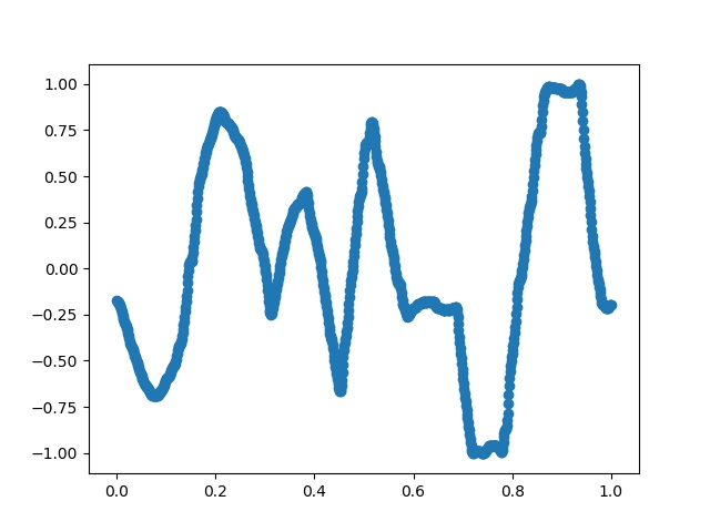
일정한 시간간격으로 추정된 위치값을 보간법으로 구해 데이터 수를 확장해 보자.

보간법

우리가 필요한 샘플링 주기는 최대 주파수 설정에 따른다.
최대 500Hz까지를 검사하여 성분 분석을 하려면 그 두배인 1000Hz를 maxfreq로 설정한다.
(나중에 나오지만 주파수 스펙트럼을 그려보면 중앙을 기준으로 좌우 대칭으로 나온다. 따라서 최대 주파수 *2를 해준다.)
1000Hz를 maxfreq로 잡으면 샘플링 주기는 1/1000 sec로 한다.
일정한 시간간격 (1ms)마다의 신호크기를 추정해 다시 그려보자.

from scipy.interpolate import splrep, splev  
  
spl = splrep(txlist[:,0], txlist[:,1])
fs = 1000 # max 500Hz *2  
dt = 1/fs   # 0.001  
spl = splrep(txlist[:,0], txlist[:,1])  
newt = np.arange(0, 1, dt)  
newx = splev(newt, spl)  
print(newt)  
print(newx)  
if True:  
    plt.figure()  
    plt.scatter(newt, newx)  
    plt.savefig('fft02_2.jpg')  
    plt.show()

FFT

위 신호를 분해해 보자.
먼저 주파수 스펙트럼을 구해서 어떤 주파수를 사용해야 하는지를 분석한다. 스펙트럼 그래프에서 높은 값을 가진 성분의 주파수를 선택하면 된다.

  
# 주파수 생성  
nfft = len(newt)  # number of sample count.  
print('nfft = ', nfft)  
df = fs/nfft    # 주파수 증가량 = max freq / 샘플개수  
k = np.arange(nfft)  
f = k*df      # 0부터~최대주파수까지의 범위 (sample count 개수 만큼, df증가량으로 분포)  
  
# 주파수 스펙트럼은 중앙을 기준으로 대칭이 된다. 반만 구한다.  
nfft_half = math.trunc(nfft/2)  
f0 = f[range(nfft_half)]      # only half size check for get hz.  
y = np.fft.fft(newx)/nfft * 2 # 증폭을 두 배로 한다. (반만 계산해서 에너지가 반으로 줌)  
y0 = y[range(nfft_half)]       # one side.  
amp = abs(y0)  # 벡터(복소수) norm 측정. 신호 강도. 
if True:  
    plt.figure()  
    plt.plot(f0, amp)  
    plt.savefig('fft02_3.jpg')  
    plt.show()

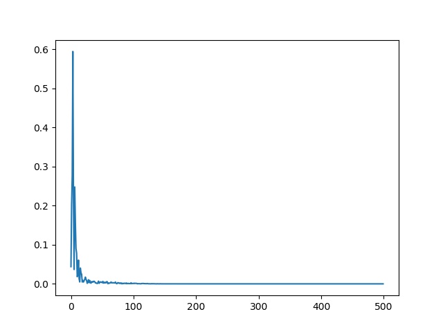
위 그래프의 가로축은 주파수이고 세로축은 신호 강도이다.
작은 값을 버리고 강도가 센 주파수만 선별하면 된다.
top N개를 설정해서 몇 개만 할 수 도 있지만, 몇 개가 최적인지 알 수 없기에 사분위수의 극단점을 이용해 보았다. (데이터 분포의 25%~75%범위의 끝에서 해당 크기의 1.5배 이상 떨어진 데이터)
굳이 이렇게까지 할 필요는 없고 특정 개수로 (예를 들면 10개로) 설정해도 된다.

  
# outlier 찾기. 사분위수 사용. boxplot.  
ampsort = np.sort(amp)  
q1, q3 = np.percentile(ampsort, [25, 75])  
iqr = q3-q1  
upper_bound = q3+1.5*iqr  
print('q1=',q1, 'q3=',q3, 'upper_bound=', upper_bound)  
outer = ampsort[ampsort>upper_bound]  
print('outer cnt=', len(outer))  
topn = len(outer)  
print(outer)

1000 개중에 특이하게 높은 값 101개를 찾았다.

nfft =  1000
q1= 2.7017249783348636e-05 q3= 0.00031241349163501486 upper_bound= 0.0007405078544125142
outer cnt= 101
[0.00081545 0.00085501 0.00086458 0.00090005 0.00090194 0.00091519
 0.00091733 0.00093784 0.00096499 0.00097396 0.00099638 0.00104299
 0.00107283 0.00126076 0.00126265 0.00127681 0.00129231 0.00131356....]

상위 101개의 주파수를 찾는다.

idxy = np.argsort(-amp)  
for i in range(topn):  
    print('freq=', f0[idxy[i]], 'amp=', y[idxy[i]])

마지막으로 주파수만으로 원본을 추정해 그려본다.

  
# recover  
newy = np.zeros((nfft,))  
arfreq = []  
arcoec = []  
arcoes = []  
for i in range(topn):  
    freq = f0[idxy[i]]  
    yx = y[idxy[i]]  
    coec = yx.real  
    coes = yx.imag * -1  
  print('freq=', freq, 'coec=', coec, ' coes', coes)  
    # newy += coec * np.cos( 2*np.pi*freq*newt+ang) + coes * np.sin( 2*np.pi*freq*newt+ang)  
  newy += coec * np.cos(2 * np.pi * freq * newt) + coes * np.sin(2 * np.pi * freq * newt)  
    arfreq.append(freq)  
    arcoec.append(coec)  
    arcoes.append(coes)  
  
plt.figure()  
plt.plot(txlist[:,0], txlist[:,1], c='r', label='orginal')  
plt.plot(newt, newy, c='b', label='fft')  
plt.legend()  
plt.savefig('fft02_4.jpg')  
plt.show()

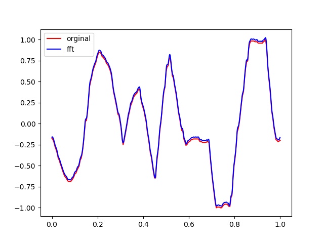
거의 복원된 모습을 확인할 수 있다.

주성분 주파수를 하나씩 추가하여 변화하는 모습을 확인해 보자.

  
# progress ...  
plt.figure()  
plti = 0  
ncnt = 15  
  
newy = np.zeros((nfft,))  
for i in range(ncnt+1):  
    freq = f0[idxy[i]]  
    yx = y[idxy[i]]  
    coec = yx.real  
    coes = yx.imag * -1  
  print('freq=', freq, 'coec=', coec, ' coes', coes)  
    newy += coec * np.cos(2 * np.pi * freq * newt) + coes * np.sin(2 * np.pi * freq * newt)  
  
    plti+=1  
  plt.subplot(4,4, plti)  
    plt.title("N={}".format(i+1))  
    plt.plot(newt, newy)  
  
plt.savefig('fft02_5.jpg')  
plt.show()

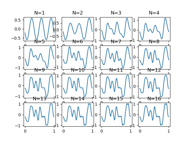
주파수를 추가할 때 마다 점점 원본의 모습으로 바뀌어진다.

Authors: crazyj7@gmail.com
Written with StackEdit.